
Statistics Behind Machine Learning: Understanding Polynomial Regression
First of all, it is a continuation of the old blog, which is "Statistics behind Machine Learning: Understand Simple Linear and Multiple Linear Regression".
Without reading that, reading this blog for those who don't know the statistics behind Simple Linear and Multiple Linear Regression feels like 'walking in a dark street'. So, read the blog first and get back here.
Now, without wasting time, let's begin.
What is Polynomial Regression?
Polynomial Regression is a type of regression technique used to model non-linear relationships between dependent and independent variables.
Instead of fitting a straight line, it fits a curve.
Why Polynomial Regression?
Many of them questioned, 'Why do we need Polynomial Regression?'
We already have Simple Linear Regression and Multiple Linear Regression.
Then why do we need Polynomial Regression?
Then why do we need this?
In one line, to handle non-linear data.
Simple and Multiple Linear Regression work well when the relationship between independent and dependent variables is linear. However, when the data follows a curved or non-linear pattern, these models tend to underfit.
Polynomial Regression addresses this limitation by transforming the input features into higher-degree polynomial terms, allowing the model to capture non-linear trends while still using a linear regression framework.
It's not a new algorithm. It's still the linear regression. But it applies polynomial transformation features.
Polynomial Regression Formula
In Linear Regression, the formula is:
In Multiple Linear Regression, the formula is:

Here, as usual, y refers to the dependent variable, b₀ refers to the intercept (c), x refers to the independent variable, and x², x³ refer to the polynomial terms.
Even though the equation looks non-linear, it is linear with respect to the coefficients. That's why it still comes under the Linear Regression family.
How are we going to use two or more inputs? First, is it possible in Polynomial regression?
Actually yes. But a small change in the formula.

Here, b₀ refers to the intercept, x and y refer to the independent and dependent variables. b₁x₁, b₂x₂ refer to the linear effect of x₁ and x₂. Simply the coefficient value. The same concept that we saw in the linear and multiple linear regression blog.
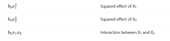
Now we get a few new terms like Squared effect and Interaction, right?
Need for Squared Effect (x²)
In Linear Regression, we assume that the relationship between input and output is constant.
That means:
If X increases by 1, Y always increases (or decreases) by the same amount.
But in real life, this assumption often fails.
For example,
- X → Study hours
- Y → Exam score
At the beginning:
1 → 2 hours of study → big improvement
Later:
8 → 9 hours of study → very small improvement
Sometimes, performance may even drop due to fatigue.
This kind of behavior cannot be captured by a straight line.
How Squared Term Helps
By adding x², the model can:
- capture curvature
- model accelerating or decelerating effects
- represent diminishing or increasing returns
So the squared term answers this question:
Does the impact of X change as X increases?
If yes, we need x².
Need for Interaction Effect (x₁ × x₂)
Now let's talk about interaction terms.
Linear Regression assumes each input variable affects the output independently. But real-world variables often work together.
For example,
- X₁ → Study hours
- X₂ → Sleep hours
Possible cases:
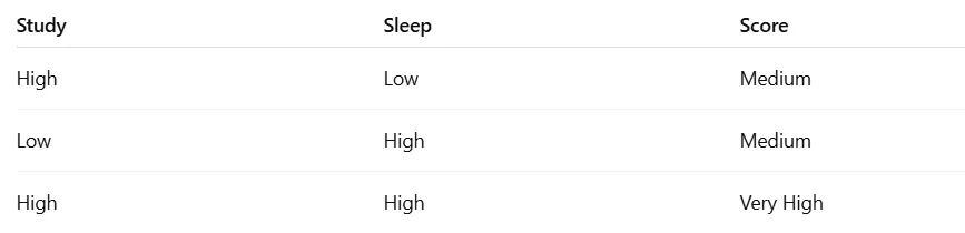
Here, study and sleep alone give moderate results.
But together, they produce the best result.
This combined influence cannot be learned using only linear terms.
How the Interaction Term Helps
The interaction term x₁ × x₂ allows the model to learn:
"The effect of X₁ depends on the value of X₂", and vice versa.
So the interaction term answers:
Does the combined effect of two variables matter?
If yes, we need interaction terms.
What Happens Without These Terms?
If we remove:
- squared terms → model stays linear
- interaction terms → model ignores combined effects
Result:
- underfitting
- poor predictions
- incorrect assumptions about data behavior
Squared terms capture the non-linear behavior of a single variable. Interaction terms capture the combined effects of multiple variables. Polynomial Regression includes both to model real-world complexity. That's why Polynomial Regression performs better than simple linear models when the data is non-linear.
Squared terms handle curvature, and interaction terms handle cooperation between variables.
Why Square? Why Not Cube? Why Not Square Root?
Here, many of them were confused.
This is a very common and genuine confusion.
Let's clear it step by step.
When we talk about Polynomial Regression, squaring is not mandatory.
We use squaring simply because it is the simplest way to introduce non-linearity.
Why Square (x²)?
Squaring helps the model capture:
- simple curvature
- smooth bending in data
- non-linear trends without too much complexity
In most real-world datasets:
- Relationships are mildly non-linear
- not extremely complex
So x² is often sufficient to model the behavior.
Also, squared terms:
- are symmetric
- easy to optimize
- less prone to extreme values compared to higher powers
That's why we usually start with degree = 2.
Why Not Cube (x³)?
Yes, we can use a cube.
But higher powers introduce:
- more complexity
- sharper curves
- a higher risk of overfitting
Using x³ means:
- The model becomes very sensitive to small changes in X
- Predictions may fluctuate wildly outside training data
So we use cubic or higher-degree terms only when the data truly demands it, and after validation.
Why Not Square Root (√x)?
Square root and logarithmic transformations are also valid, but they serve a different purpose.
They are usually used when:
- Data grows very fast initially then slows down quickly
- or when variance needs stabilization
Polynomial Regression focuses on feature expansion, not transformation.
So √x is more common in:
- data preprocessing
- normalization
- variance stabilization
Not as a default polynomial term.
Who Decides Which Power to Use?
Not humans.
Not assumptions.
The data decides.
We choose the degree by:
- checking model performance
- using validation data
- observing underfitting vs overfitting
In practice:
- start with degree = 2
- increase only if needed
- stop when performance drops
Python Code
import numpy as np
from sklearn.preprocessing import PolynomialFeatures
from sklearn.linear_model import LinearRegression

X = [
    [2, 6],
    [3, 5],
    [4, 4],
    [5, 3]
]

y = [50, 60, 70, 80]

X = np.array(X)

poly = PolynomialFeatures(degree=2)
X_poly = poly.fit_transform(X)

pr = LinearRegression()
pr.fit(X_poly, y)

predicted = pr.predict(poly.transform([[4, 4]]))[0]
print(f"Predicted value is: {predicted}")
Step 1: Dataset
import numpy as np
from sklearn.preprocessing import PolynomialFeatures
from sklearn.linear_model import LinearRegression

X = np.array([
    [2, 6],
    [3, 5],
    [4, 4],
    [5, 3]
])

y = np.array([50, 60, 70, 80])
Here:
- Column 1 → X₁
- Column 2 → X₂
Step 2: Polynomial Feature Transformation
poly = PolynomialFeatures(degree=2)
X_poly = poly.fit_transform(X)
Now internally, X becomes:
[1, x1, x2, x1², x2², x1*x2]
You don't see it, but it's happening 😄
Step 3: Train the Model
pr = LinearRegression()
pr.fit(X_poly, y)
Behind the scenes:
- Statistics calculates all coefficients
- Finds the best curve/surface
Step 4: Prediction
predicted = pr.predict(poly.transform([[4, 4]]))[0]
print(f"Predicted value is: {predicted}")
Here, we predict the output for X₁ = 4, X₂ = 4
Important thing to note:
- We give only original input values
- PolynomialFeatures automatically transforms them before prediction
Output
Predicted value is: 70
When you see deeply, the entire concept and working model in the polynomial regression is similar to the simple and multiple linear regression. The only difference is using the nth degree to handle non-linear data.
So, I hope the blog helps you to get the insight about Polynomial Regression, behind statistical works, and Python code.